Simple Expenditure Spreadsheet Example.

1. Getting Started.

A Spreadsheet does the same job as ledgers and account books do. Spreadsheets are composed of columns under letters and rows after numbers. Every cell or box in a spreadsheet can be identified by cross reference to these numbers and letters; A1 or C6
Start OpenOffice Spreadsheet.
To make it really easy, we will start by adding up a sum of numbers.
Let's assume that you spend some money each day on different items and that you want to keep track of your expenditure.
In the first cell (A1), type the word DAY. You can change the format and font later if you wish
Notice that as you type the word DAY, it also appears in the Input Box above the letters. Clicking on any cell, makes its contents appear in the Input Box. This makes editing easy and straightforward
Underneath the word DAY, in the cell A2, type SUNDAY, and press enter.
Click on the box (A2) again. Move your mouse to bottom right corner of the cell until the cursor changes to a plus sign. Now click and drag your mouse downwards for the next 6 cells. You will notice that the days of the week are filled in automatically.
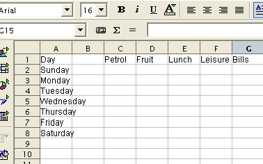
Your spreadsheet should look like this:
Now in Cell C1, type the word Petrol. Press enter. Type similar expenditure items in the next four cells.

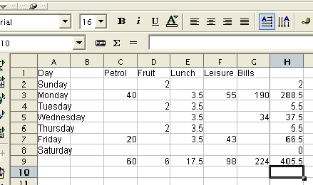
Now underneath the word PETROL, put in any amount in numbers for any particular days. Do not put in any currency sign at this stage. Fill in the other cells in a similar fashion.
You will notice that figures do not look well without the correct formatting. We will correct this later.

Now we will total each column and row. Click on cell C9. Type =Sum(C2:C8) exactly as it is here. The = sign means that you expect to perform a calculation, in this case a sum. Press ENTER. If you used my figures, the number C9 should change to 60.
Instead of totaling each column separately, you can use click and drag. Click on cell C9, move the mouse to the bottom right hand corner of this cell until the cursor changes to a plus sign. Click and drag to the right until you reach cell G9. The column totals appear automatically.
Now click on cell H2 and and type =sum(C2:G2). Press ENTER. As there is only one item in this row, the H2 cell should show a total of 2. Now click on the H2 cell again. Move the mouse to the bottom right hand corner of this cell until the cursor changes to a plus sign. Click and drag downwards until you reach cell H9. This will total all the other rows.
Now each column and row is totaled and it is easily possible to see how much you spent on each area or on each day. The total expenditure for the week was 405.5.

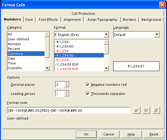
Now some formatting is necessary. Click on Cell C2 and drag to select the entire area from cell C2 to H9. Now choose FORMAT from the top line menu, then choose CELLS. From the options presented, chooses NUMBER. Here you can choose the currency.
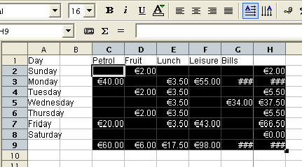
Click OK when you have chosen the currency and decimal places. Some numbers may change to #### signs when you do this. This is because there is no longer room for the entire number including its decimal places in the cell.
To overcome this problem, select the entire area again. Choose FORMAT from the top line menu, click on COLUMN and OPTIMAL WIDTH. This should allow the correct amount of space for each number.
The huge benefit is the ability to change any expense within the week to any other number. All the totals change accordingly. Try this and see.

Last modified: 2008-04-30 01:42 UTC

This work is licensed under a Creative Commons Attribution2.5 License.